Fluid Statics
- Absolute and gauge pressure
- Pressure vs depth at constant density
- Pressure in the atmosphere
- Measuring Pressure
- Pascal’s law & Hydraulic systems
- Hydrostatic forces on submerged surfaces
Our discussion of fluid pressure began in the previous chapter. As a reminder, Pressure is the force applied perpendicular to a surface per unit area. When we speak of pressure we are typically dealing with a gas or a liquid that is confined to a container.
\[\mathrm{Pressure}=\frac{\mathrm{Force}}{\mathrm{Area}}\,, \qquad\qquad p=\frac{F}{A}\]In the SI system a force per unit area has units of newtons per square meter $\N/\m^2$, which is called the pascal ($\Pa$). In the USCS a force per unit area has units of pound per square foot, $\lb/\ft^2$, abbreviated as psf. For fluids, it is more convenient and customary to express pressure in units of pounds per square inch, $\lb/\inch^2$, abbreviated as psi. For the remainder of this course we will use psi as the standard unit of pressure when working in the USCS of units.
Absolute and gauge pressure
The pressure when measured relative to an absolute vacuum is called the absolute pressure. In practice a near absolute vacuum is difficult to obtain. Therefore most pressure-measuring devices record pressure relative to the local atmospheric pressure. In this design the pressure gauge is calibrated to read zero when it is at atmospheric pressure and the pressure indicated is actually the difference between the absolute pressure and local atmospheric pressure. This difference is called the gauge pressure and can be expressed as
\[p_{\rm absolute}=p_{\rm gauge}+p_{\rm atm}\]The figure below summarizes the relationship between gauge and absolute pressure measurements.

An automobile tire is inflated to a pressure of 30 psi (gauge). Determine the absolute pressure in the tire.
To find the absolute pressure we use the expression
\[p_{\rm absolute}=p_{\rm gauge}+p_{\rm atm}\]Since the atmospheric pressure wasn’t explicitly stated we use the standard value of 14.7 psi. The absolute pressure inside the tire is
\[p_{\rm absolute}=30~\psi+14.7~\psi=44.7~\psi\]Pressure vs depth at constant density
The pressure in a fluid increases with depth simply because more fluid sits above the deeper layers of fluid. In order for the deeper layers of fluid to support the increasing weight resting above it, the pressure of the fluid must increase accordingly. For a static, homogenous, incompressible fluid the relationship between pressure and depth is
\[\Delta p = -\gamma \Delta z\]where $\Delta p$ is the change in pressure that occurs across an elevation change of $\Delta z$. $\gamma$ is the specific weight of the fluid. The minus sign indicates that a decrease in elevation causes an increase in pressure. In practice I just calculate the magnitude of the change in pressure (ignore the minus sign) and afterwards determine whether the pressure decreased (increase in elevation) or the pressure increased (decrease in elevation). Just remember that as you increase the amount of fluid above you, the fluid pressure will also increase.
Compute the change in pressure as you descend to the bottom of an 8 foot deep pool.
We use the formula $\Delta p = -\gamma \Delta z$ but I will compute it without the minus sign (take the absolute value).
\[\Delta p = \left(62.4~\frac{\lb}{\ft^3}\right) \times\left(8 ~\ft\right)=499.2~\frac{\lb}{\ft^2}=499.2~{\rm psf}\]Now convert to the customary psi
\[499.2~\frac{\lb}{\ft^2}\times\left(\frac{1~\ft}{12~\inch}\right)^2=3.47~\psi\]As one descends to the bottom of the pool the pressure increases by about 3.5 psi. This is an increase above atmospheric pressure by about 20%. (Atmospheric pressure is 14.7 psi.)
Here is another example.
A hiker’s barometer reads 95 kPa at the beginning of her trip and 85 kPa at the end. Assuming a constant air density of $1.22~\kg/\m^3$ estimate the vertical distance traversed by the hiker. Was the hiker climbing or descending?
Let’s first determine whether the hiker was climbing or descending. The pressure was larger at the start of the trip. In order for the pressure to decrease the hiker must have been ascending. As the hiker increases her altitude there is less air above her, compared to when she started. This results in a decrease in pressure.
The net change in pressure is 10 kPa which is 10,000 Pa. The specific weight of air can be computed from the density
\[\gamma=g\rho=(9.81~\m/s^2)\left(1.22~\kg/\m^3\right)=11.97~\N/\m^3\]We can rearrange the pressure elevation relationship to solve for $\Delta z$. (Again, I dropped the minus sign since we already know the hiker is climbing.)
\[\Delta z = \frac{\Delta p}{\gamma}=\frac{10,000~\Pa}{11.97~\N/\m^3}=836~\m\]So the hiker made a net vertical ascent of 836 meters.
Pressure in the atmosphere
The previous exercise incorporated an important assumption, that the air density remains constant throughout the 800 meter ascent. This is not entirely realistic. The temperature of the air changes with altitude and therefore so must the density (think ideal gas law). In order to simplify our discussions we will make use of the 1976 U.S. Standard Atmosphere. In this model the atmosphere is broken up into seven layers with each layer having a prescribed linear temperature profile.
Starting from the sea level properties of air (see table below) one can compute other relevant properties, but the procedure goes beyond the scope of this course. Instead, the properties of air at various altitudes should be found by using the 1976 U.S. Standard Atmosphere Calculator.
| Property | Symbol | SI | USCS |
|---|---|---|---|
| Temperature | $T$ | $15\C$ | $59\F$ |
| Pressure | $p$ | 101.3 kPa (abs) | 14.7 psia |
| Density | $\rho$ | $1.22~\kg/\m^3$ | $2.377\times 10^{-3}~\slug/\ft^3$ |
| Dynamic viscosity | $\eta$ | $1.789\times 10^{-5}~\Pa\cdot s$ | $3.737\times 10^{-7}~\lb\cdot s/\ft^2$ |
A drive to the top of Mt. Washington begins at an elevation of 1600 ft. The tire pressure, as measured with a standard tire pressure gauge, is 30 psi at the start of the trip. What will the tire pressure gauge read at the end of the trip at an elevation of 6200 ft. Work under the assumption that the air in the tires remain at the same temperature.
The important thing to note is that a standard tire pressure gauge is measuring a gauge pressure. So the pressure measurement of 30 psi means that the tire is 30 psi above the ambient pressure.
Our trip starts at an elevation of 1600 ft. Using the 1976 U.S. Standard Atmosphere Calculator the ambient air pressure is 13.9 psi. The absolute pressure in the tire is therefore
\[p_{\rm absolute}=p_{\rm gauge}+p_{\rm atm}= 30~\psi + 13.9~\psi = 43.9~\psi\]Arriving at the top of Mt. Washington the absolute pressure in the tire remains 43.9 psi.
Using the 1976 U.S. Standard Atmosphere Calculator we find that the atmospheric pressure has now dropped to 11.7 psi. When making a measurement of the gauge pressure we find
\[p_{\rm gauge}=p_{\rm absolute}-p_{\rm atm} = 43.9~\psi - 11.7~\psi = 32.2~\psi.\]So the tire pressure increases by 2.2 psi. This is the pressure that dictates how the tires will handle.
Note the huge assumption that the temperature of the air remains unchanged. This is unlikely to be the case. One rule of thumb is that for every $10\F$ increase in temperature the pressure increases by 1 psi. So if the temperature dropped by $20\F$ throughout the course of the trip it would compensate for the increase from change in atmospheric pressure.
Measuring Pressure
Manometers
One of the most basic pressure measurement devices is the manometer. A simple U-tube monometer is shown in the figure below. One end of the manometer is connected to a fluid of unknown pressure. In the example below we want to find the pressure of the water at point $A$. The other end of the U-tube manometer is open to atmospheric pressure. A gauge fluid, that does not mix with the fluid to be measured, sits between the two. Typical gauge fluids include Mercury (as used in this example), colored light oils, or water.

Compute the pressure at point A using the manometer shown above.
Start at the point labeled $1$ where the pressure is the atmospheric pressure,
\[p_1=p_{\mathrm{atm}}=0~\kPa~\mathrm{(gauge)}\]We now move to point $2$. The pressure there is higher than that of point $1$ due to the gauge fluid sitting above it. Using the pressure-elevation relationship we see that the pressure at 2 is larger by $\gamma_{m} (40~\mm)$, where $\gamma_{m}$ is the specific weight of mercury.
\[p_2=p_1+\gamma_{m} (40~\mm)\]Because points $2$ and $3$ are at the same height, at rest, and within the same fluid the pressures are equal, $p_3=p_2$. Next we go to point $4$. The pressure at $4$ is lower than the pressure at $3$ by an amount $\gamma_w (70\mm)$ where $\gamma_w$ is the specific weight of water.
Finally, because point $A$ and $4$ are at the same elevation their pressures are the same.
\[p_4=p_A=p_1+\gamma_{m} (40~\mm)-\gamma_w(70~\mm)\]Using
\[\gamma_w=9.81~\kN/\m^3\,,\quad\quad \gamma_{m}=(13.54)(9.81~\kN/\m^3)=132.8~\kN/\m^3\]we can solve for the pressure at point $A$:
\[p_A=0~\kPa~\mathrm{(gauge)} + 132.8~\kN/\m^3 (0.04~\m) - 9.81~\kN/\m^3 (0.07~\m)=4.63~\kPa~\mathrm{(gauge)}\]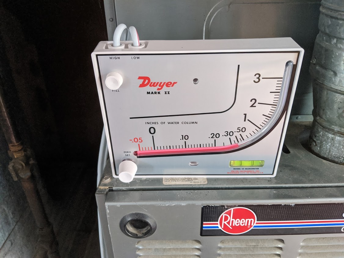
Dwyer Mark II inclined manometer measuring slightly less than 0.4 inWC. The manometer measures the pressure drop across an air filter. As the air filter accumulates dust over time the pressure drop across it increases. The inclination of the tube allows for a more sensitivity at lower pressures.
Barometers
A barometer is used for measuring the atmospheric pressure. In its simplest form it consists of a long tube closed at one end that is filled with mercury. When the open end of the tube is submerged into a container of mercury a near perfect vacuum is produced at the closed end.

If we analyze the above barometer in the same manner as a manometer we can derive the relationship
\[p_{atm}=\gamma_{m} h\]For example, let’s say that a mercury barometer measured a height of $h=760~\mm$. This would correspond to an atmospheric pressure of
\[p_{atm}=\frac{133.3~\kN}{\m^3}\times 0.760~\m=101~\kPa\]Pressure expressed as a height of liquid
It is sometimes convenient to express pressure as a height of a column of fluid. For example, instead of stating the atmospheric pressure as 101 kPa we could have said the pressure is 760 mm of mercury. Of course, “mm of mercury” is not a unit of pressure, but when stated as such we should know to interpret this as the pressure that would cause a rise of 760 mm of mercury in a barometer.
For example, a pressure of 1.0 mm of mercury (mmHg) corresponds to a pressure $p=\gamma h$
\[\text{1.0 mmHg}=\gamma_{m}h=\frac{133.3~\kN}{\m^3}\times 0.001~\m = 0.1333~\kPa = 133.3~\Pa\]For smaller pressure inches of water (inH$_2$O or inWC), the WC stands for water column, is used instead of psi.
\[\text{1.0 inH}_2\text{O}=0.0361~\psi\]Pressure gauges
A mechanical pressure sensor coverts fluid pressure into a force that displaces a flexible element. The movement in the element moves a dial which, after calibration, serves as a visual indication of the pressure. Three common styles of mechanical pressure sensors are sketched below.
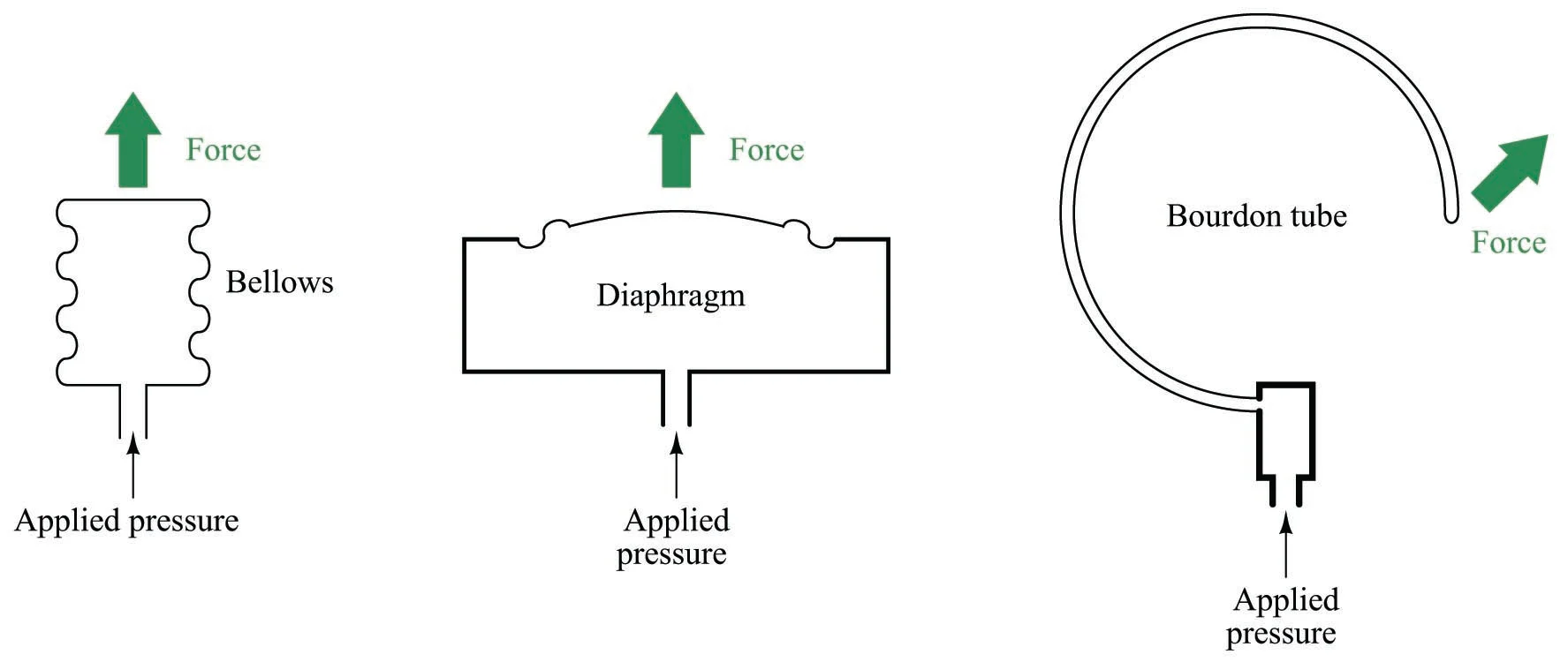
The bellows, the diaphragm, and the bourdon tube. From: Mechanical Pressure Elements licensed under CC BY 4.0.
Video: Bellows For Pressure Sensing
Video: How a Bourdon tube works
Video: Diaphragm element compared to Bourdon tube
Pascal’s law & Hydraulic systems
Pascal’s law states that if there is a pressure change at some point in a confined incompressible fluid, there is an equal change everywhere else in the fluid. In the following example we will make use of Pascal’s law to show how a hydraulic lift can be used to magnify forces.

In the above figure a force $F_1$ is applied to the left piston which has an area $A_1$ in contact with the fluid. This produces a pressure $p=F_1/A_1$ in the fluid. Pascal’s law states that this pressure is transmitted everywhere else in the fluid, for example to a point just under the large piston on the right. In other words, the pressure everywhere in the fluid is the same.
Therefore, if we are in static equilibrium (the pistons aren’t moving), the force applied to the right piston, $F_2$, must produce the same pressure in the fluid, $p=F_2/A_2$. We therefore have that
\[\frac{F_1}{A_1}=\frac{F_2}{A_2}\]or
\[F_2= \frac{A_2}{A_1} F_1\]The quantity $A_2/A_1$ is called the mechanical advantage.
A car weighing 2000 pounds is supported on the hydraulic lift shown below. What weight, $w$, is needed on the piston on the left in order to support the car? What is the pressure, in psi, of the hydraulic fluid?

The ratio of the areas of the two pistons is the mechanical advantage. The force required to the support the car is a factor of 10 less.
\[F_1=\frac{A_1}{A_2}F_2=\frac{10~\ft^2}{100~\ft^2}\times 2000~\lb=200~\lb\]The pressure in the hydraulic fluid is
\[p=\frac{F_2}{A_2}=\frac{2000~\lb}{100~\ft^2}\times\left(\frac{1~\ft}{12~\inch}\right)^2=0.14~\psi\]Note that we could have computed the pressure using $p=F_1/A_1$ and obtained the same result.
Hydrostatic forces on submerged surfaces
Consider the retaining wall shown below. The fluid pressure on the wall increases from zero at the surface of the fluid to a maximum pressure at the bottom. The pressure elevation relationship, $p=\gamma h$, tells us that the pressure increases linearly with depth.
The resultant force on the load is equal to the area under the pressure distribution times the area of the wall. The average pressure on the wall is $p_{avg}=\gamma h/2$ and the magnitude of resultant force is
\[F_R= p_{avg}\times A=\gamma \left(\frac{h}{2}\right) A\]where $A$ is the surface area of the wall that is in contact with the fluid. The location of the resultant force is located at the center of pressure a distance $h/3$ from the bottom of the wall.

A 10 foot wide gate is supported by a horizontal cable as shown in the figure. Water acts against the gate which is hinged at its bottom. What is the tension in the cable. You can neglect any friction in the hinge.

We start by drawing a free body diagram of the gate. The forces on the gate include the fluid pressure, the reaction forces from the hinge acting on the gate, and the tension from the cable.

Left: Free body diagram of the gate. The tension force from the cable is $T$. The force distribution from the water is shown in red.
Right: Equivalent free body diagram of the gate. The force distribution from the water is replaced by the single resultant force $F_R$ located a distance of 5 feet from the bottom.
The resultant force on the gate is the average pressure, $p_{avg}=\gamma h/2$ times the area of the gate in contact with the fluid. In this example that area is $A=15~\ft \times 10~\ft = 150~\ft^2$.
\[F_R= \gamma \left(\frac{h}{2}\right) A=62.4~\frac{\lb}{\ft^3} \left(\frac{15~\ft}{2}\right) 150~\ft^2=70,200~\lb = 70.2~\textrm{kip}\]To find the tension in the cable we set the sum of the moments about the hinge to zero. I’m using the convention that a counter-clockwise moment is positive.
\[\sum M_O=F_R\times 5~\ft-T\times 18~\ft=0\] \[T=\frac{5~\ft}{18~\ft} \times F_R = 19.5~\textrm{kip}\] |
About
|
Back to Applied Fluid Mechanics Resources & Notes
|
About
|
Back to Applied Fluid Mechanics Resources & Notes